CatchmentSIM Help

 

Download Tutorial 5 Data and Solution File

 

Tutorial 5 shows how to develop a CatchmentSIM project for a network of non-dendritic (i.e., closed) watersheds in Western Florida. The tutorial shows how to setup a DEM using LiDAR data, condition the DEM so that depression areas are preserved, calculate stage-area-storage relationships, and calculate SCS runoff curve numbers using soils and land use GIS layers.  

 

 

SETUP Project

 

To begin a new project, select CatchmentSIM Drop Down >> New Project.

 

Enter any relevant information in the Project Information text fields (these can be left blank if you wish).

 

Click the "Browse" button and enter the filename and location of your project. Your CatchmentSIM project should ideally be located in the same folder or above the folders that contain all of the input data (e.g., LiDAR) and external GIS files that you will use to develop your CatchmentSIM project.  

 

You should now select the relevant projection / coordinate system for your project. Click the Set Projection button and select "U.S. State Plane Coordinate Systems (1983, feet)" from the "Projection Class" field and then select "Florida 0902, Western Zone (1983, US Survey Feet)" from the "Projection Sub Class" field.

 

Next, enter the X & Y design plane extents for the project. The region defined by these coordinates is the design plane and all source data will be clipped at its intersection with this plane. This ensures that file sizes and processing times are minimised.  

 

Enter the following design plane coordinates in the boxes:

 

Xmin: 485000

Ymin: 1660000

Xmax: 490000

Ymax: 1665000

 

The scaling factors near the bottom of the New Project form enable coordinate systems and elevations scales that are not in metric m x m grid formats to be used with CatchmentSIM. In this case, the coordinate system and elevations are in feet and hence the scaling factors should be automatically updated to 3.280833.

 

The default area, length and volume units can also be set at this time.  Set the default length units to "Feet", the area units to "Acres", the default percentage units to "%", and the volume units to "M ft3".

 

The completed New Project form should look similar to the following (you may or may not have data in the Project Information section of the form):

 

 

Click "OK".

 

 

developing the dem

 

For this Tutorial we will develop a DEM using a LiDAR (Light Detection And Ranging) LAS data file.  

 

First a blank DEM (i.e., a DEM with no elevations assigned) must be developed. To setup a blank DEM, select Create DEM >> Setup Blank DEM. Select the "Use Design Plane" radio button to set the DEM extents to the design plane extents.  Ensure that the "Use Square Grid Cells" check box is selected and select the "2b) Set Cell Size (Square Cells Only)" radio button. Enter "5" in the text box to specify a raster grid size of 5 feet x 5 feet.  The completed form should look similar to the following:

 

 

Now we must assign elevations to each DEM pixel (i.e., cell) using a LiDAR data file. To import the LiDAR data file, select Create DEM >> Spot Heights and select "LAS (LiDAR) Data File (*.las)" from the file type drop down box. Select the LiDAR data file for import, in this case "LiD2006_10480.las".  

 

In addition to containing elevation information, LiDAR LAS data files also include data point classifications (e.g., ground points, vegetation, buildings). CatchmentSIM will read the LiDAR data file to identify all of the different data point types that are available.  After CatchmentSIM has read the LiDAR data file, a dialog box will appear which will allow you to select which data point types you would like to use to populate your DEM. For this LiDAR data file, two different data point types are available; "Unclassified" and "Ground". As we are interested in defining watershed boundaries and flow paths for the natural ground surface we will just use the ground points. Uncheck the "Include All Available Classes" check box near the top of the form. Also uncheck the "Unclassified" data point type in the 'Include' column so that only "Ground" point types are checked, as shown below.

 

 

Click "OK". A "Dataset Projection" dialog will appear asking if the LiDAR data file is in the same coordinate projection as the CatchmentSIM project.  If you select "No", CatchmentSIM will ask you to specify the projection of the LiDAR file and it will perform all of the necessary coordinate conversions so that the LiDAR data file overlays the design plane correctly.  For this tutorial, the LiDAR data is in the same projection as the design plane, so you can select "Yes". After selecting "Yes", CatchmentSIM will extract just the ground points from the LiDAR data file and will use these points to populate the DEM.

 

The DEM should appear similar to that shown below.  As you can see, elevations have been assigned to the majority of the DEM.  However, some 'white space' remains in areas where no ground data points were available (e.g., buildings, vegetation).  

 

 

 

 

interpolation of the dem

 

Now we must assign elevations to the remaining 'white space' (i.e., DEM cells without any elevations). This is achieved by interpolating their values from surrounding pixels.

 

Select Create DEM >> Interpolation Tools >> Interpolate Remaining Areas. Retain the default corner elevations at the top of the 'Interpolate Digital Elevation Model' form. Next we must select the number of search rays to use for the interpolation. The number of search rays indicates the number of directions the interpolation algorithm will look in when searching for nearby assigned pixels. The higher the value you select, the more reliable the DEM will be and the longer the interpolation will take.  However, as we only have a relatively small number of unassigned pixels, we can select 32. Press "OK".

 

Following interpolation of the DEM, you should see that all DEM pixels have been assigned elevation values, as shown below.

 

 

 

hydrologic treatment of dem

 

Although the DEM has now been developed, it may not yet be ready for use to delineate the watersheds. The DEM will probably contain localised flat or depression pixels, that is, pixels that are either equal or lower in elevation than the lowest of their neighbouring pixels.

 

Flat and depression pixels can be displayed by selecting 'Flats and Pits' in the Layer Controller. As shown in the image below, isolated flat pixels (red pixels) and depression pixels (blue pixels) occur across the DEM, which can impact on hydrologic connectivity. CatchmentSIM includes three different algorithms to fix this problem and ensure smooth drainage paths over the DEM. The algorithms are referred to as the filling algorithm, the breaching algorithm and the pit algorithm, and can be used in isolation or in combination to rectify unwanted flat and depression pixels.

 

 

As we are analysing a deranged (ie., closed) drainage network, some of the flat and depression pixels serve as "sinks" or watershed outlets. These may be natural depressions, stormwater pits, stormwater ponds and/or lakes. These areas must be preserved if the flow path, watershed boundary and storage characteristics of the depression are to be reliably replicated.  Therefore, we must condition the DEM so that isolated flat and depression pixels that do not serve as outlets are removed, but flat and/or depression pixels that would actually serve as outlets are retained.

 

This could be achieved using either the breaching algorithm or the pit algorithm.  The filling algorithm is not suitable for deranged drainage networks as it has the potential to fill some depression areas, which may impact on the reliability of delineated watershed boundaries as well as any stage-area-storage calculations. However, a selective filling algorithm could be applied, which only fills some depressions areas based on user defined criteria. For further information on the selective filling process, please refer to 'Hydrologic Conditioning on Non-dendritic Drainage Terrains'.

 

In order to use the pit algorithm, it is necessary to first define watershed outlets so that flat and depression pixels representing watershed outlets are preserved (the outlet locations can be digitised onscreen or imported from an external GIS file).  As we do not have any watershed outlet information for the study area, we will use the breaching algorithm in conjunction with a maximum elevation change to ensure that major depression areas are preserved.

 

To select the breaching algorithm, select DEM Conditioning >> Breaching Algorithm. The breaching algorithm dialog will appear. Ensure that the "Use Max Elevation Gain" check box is selected and set this value to 3.0 feet.  Any flat or depression pixels that require pixel elevations to be changed by 3 feet or greater will not be altered. This will ensure that major depression areas will be retained.

 

Also set the Breaksize to a large value (20,000 should be suitable).  This will increase the available search space, which will help to ensure that the algorithm will find a solution (this will generally lead to an increase in processing time).  The completed form should look similar to the following:

 

 

Click the "Process Entire DEM" button to start the algorithm.  When applying the breaching algorithm to other projects, you may need to apply the algorithm several times using progressively higher maximum elevation gain values until acceptable results are achieved.  

 

After completion of this algorithm you should notice that flat and depression pixels have been mapped to an optimised downslope outlet pixel and this is indicated on screen by a yellow line (only those pixels requiring elevation changes of less than 3 feet have been rectified by the algorithm). Pixel elevations along this line have been linearly lowered to provide a downslope flow path for the original flat or depression pixel. If you redraw the screen (F2) and re-map flat and depression pixels you should now notice that only single isolated depression pixels are retained within actual depression areas (typically stormwater ponds).

 

 

WATERSHED BOUNDARY DELINEATION

 

At this stage your DEM should be ready for use in delineating watershed boundaries. To test flow routing on the DEM try mapping flow from a selection of pixels across the DEM. Do this by selecting Flow Mapping >> Map Pixel Flow Path and clicking on some points on the screen. As shown in the diagram below, you should see the downslope flow path of these pixels mapped until they reach a stormwater pond or other depression area.

 

 

As discussed, the flat and/or depression pixels that remain after conditioning the DEM will actually serve as watershed "sink" or outlet locations.  To define these flat and depression pixels as watershed outlets, select Subcatchments >> Other >> Add Flats and Pits as Outlets.  A form will appear which enables the user to specify a Cluster Tolerance as well as an optional Target Zone. If the Target Zone check box is selected, the user can select a polygon GIS file and only those flat and depression pixels falling within the polygon will be added as outlets. We will not set a Target Zone for this example and we will retain the default Cluster Tolerance value of 30.  The Cluster Tolerance value is used to specify that all flat or depression pixels that fall within 30 pixels of another flat or depression pixel will not be considered as a separate outlet. This will ensure that  any remaining pixels located in close proximity to one another will be considered as one single outlet.

 

Click "OK". The watershed outlets have now been defined.

 

Now we can delineate the watershed boundaries.  This is completed by selecting Subcatchments >> Map All. This is one of the most time-consuming algorithms in the program as it is effectively drawing flow path maps for every pixel in the DEM and recording which ones flow through the pixels you have designated as outlets.

 

A message box will appear stating that since you have multiple separated catchments, would you like to switch to integer based labeling.  Select "Yes".

 

Following completion of the flow processing, the watershed boundaries should appear as shown below (try changing the line colour/thickness or turning off the DEM background using the Layer Controller if you are having trouble seeing it). Problems with any flat or depression pixels within the  DEM will become obvious at this stage and should appear as holes in the watersheds. You can also see that the reliability of the watershed boundaries around the perimeter of the DEM are less well reproduced as we are "truncating" the boundaries to the limits of the DEM. If more reliable definition of these perimeter watersheds is required, we would need to increase the extent of the design plane and complete the above steps again.  However, for this tutorial the delineated watersheds are satisfactory.

 

 

 

Watershed overflow locations and directions

 

Watersheds that are delineated in CatchmentSIM are automatically labelled and arranged in a hydrologic network arrangement. However, in the case of a deranged drainage network, each watershed is typically self-contained and functions as a hydrologically separate entity in most small rainfall events. That is, the watersheds are not typically linked together. However, during more severe storms there is potential for rainfall to fill each depression area and spill into an adjoining basin.  CatchmentSIM automatically calculates the location and elevation of the watershed overtopping point.  The overflow pixel, ponding depth at the point of overtopping, downstream watershed ID and overflow elevation can be obtained in the Subcatchment Manager, which can be opened by selecting Subcatchments >> Subcatchment Manager (note that it may be necessary to customise the Subcatchment Manager form in order for this information to be displayed).

 

 

CatchmentSIM also maps watershed overflow locations and directions visually. To view this select "Nodal Link Arrangement" in the Layer Controller. The nodal link arrangement for the tutorial is shown below. The numbers in the image below refer to the watershed ID numbers and the arrows show the direction of flow from one watershed to another if their storage capacity is exceeded.

 

 

 

Background Imagery

 

CatchmentSIM supports a wide range of raster background imagery. This tutorial includes a MrSID aerial image. To load the MrSID image, select the green add button on the Layer Controller and select the "q4021se.sid" image. A message box will appear asking if the coordinate projection of the image is the same as the CatchmentSIM design plane. Select "Yes".

 

If you now click the "Apply" button the aerial image will appear. However, the DEM will disappear as the image now overlays it. This can be rectified by making the image partially transparent.  This is achieved by clicking on the image in the Layer Controller and clicking on "Properties". The Edit Raster Layer form will appear. Ensure that the "Use Transparency" check box is selected, set the transparency to 50% and click "Apply".  Both the DEM and the aerial image should now be visible, as shown below (note that the watershed boundary colour has been modified to improve contrast and the nodal link arrangement is deselected).

 

 

 

 

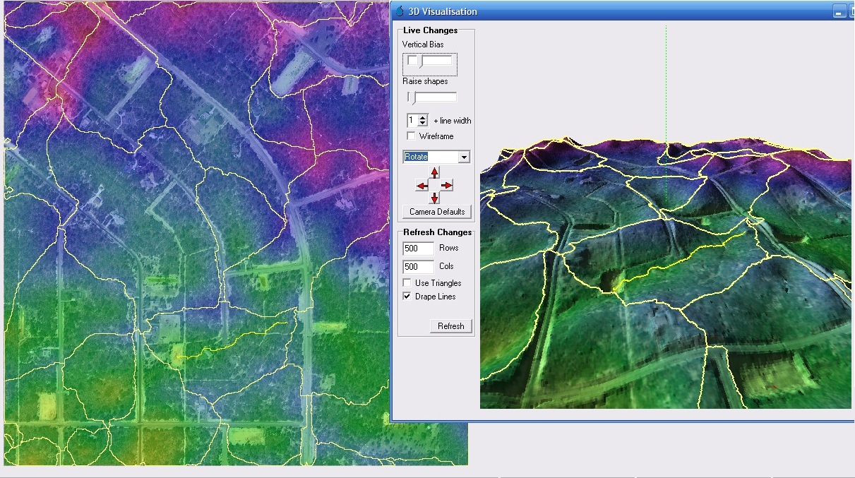
3D Visualisation (ADD ON MODULE)

 

CatchmentSIM includes an optional visualisation module that allows any raster or vector layer in CatchmentSIM to be displayed using 3D OpenGL graphics. To open the 3D visualisation module select Utilities >> Show 3D Viewer.  The visualisation module can be navigated by using the left and right mouse buttons. Hold down the left mouse button and move the mouse to rotate the view. To zoom in and out, hold down the right mouse button and move the mouse left and right.

 

You will notice that the terrain across the project area provides limited topographic relief. To improve the visualisation we can apply a vertical exaggeration by moving the "Vertical Bias" slide bar to the right.  The "Raise Shapes" slide bar car also be shifted slightly to the right to avoid the basin boundaries disappearing behind hill crests. The resolution of the 3D image can also be improved by increasing the number of Rows and Columns from 200 to 500 (for example).  However, this does require more processing time.

 

The 3D visualisation engine is tightly integrated within CatchmentSIM's graphic engine and it can be viewed in tandem with the normal 2D plan view during normal operations. For example, the Draw Pixel Flow Path operation will be rendered on both the 2D and 3D views simultaneously, as shown below by the yellow line. The 3D display settings (e.g., colours) are the same as those set for the 2D map and may be edited in the Layer Controller.

 

 

 

stage-area-storage relationships

 

Hydrologic models of deranged drainage systems typically require stage-area-storage information to define the available floodplain storage capacity of depression areas. CatchmentSIM can automatically develop stage-area-storage relationships based on the DEM and polygon boundaries defining the extent of each storage area. In deranged drainage systems, the watershed boundaries typically define the extent of each storage area.

 

To calculate stage-area-storage calculations for each watershed, we must add the watershed boundaries as lakes in CatchmentSIM.  This  is achieved by selecting Subcatchments >> Add Lakes >> Add All Subcatchments As Lakes. A blue opaque surface will extend across all areas where stage-area-storage relationships will be calculated.  To turn off or modify the blue surface so that the other vector and raster layers remain visible, de-select or edit the Lakes vector layer in the Layer Controller.

 

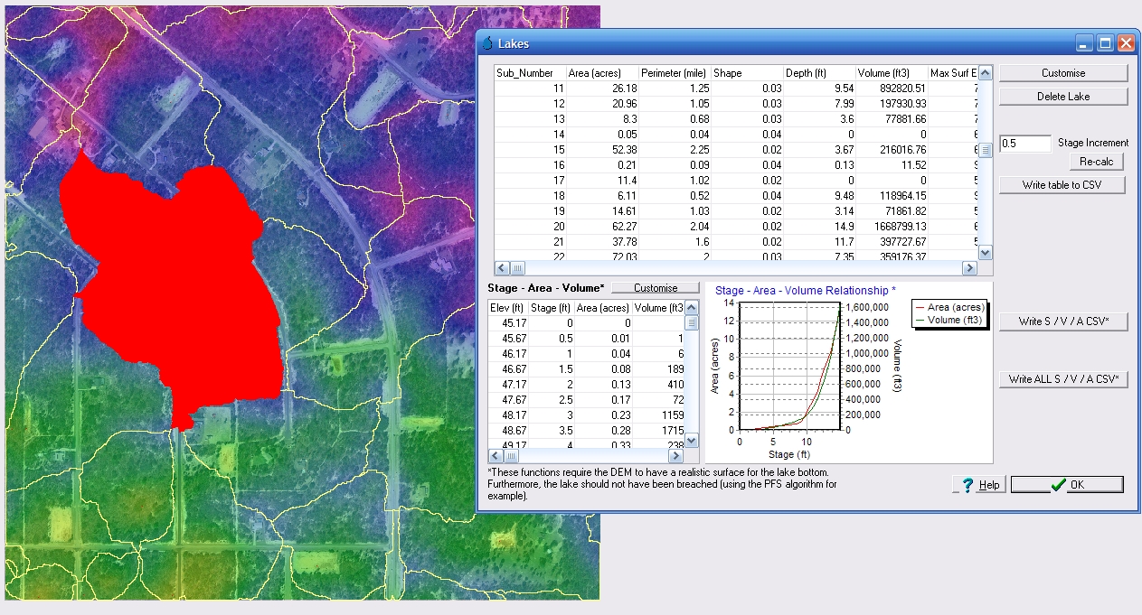
To view the stage-area-storage relationship for each watershed, open the Lake Database by selecting Subcatchments >> Lakes Manager. The top table in the Lakes Database summarises the stage-storage details for each depression area in the project.  If you click on an individual row in the top table, the watershed that this row corresponds to is highlighted in red in the 2D plan window, as shown below.  The detailed stage-area-volume characteristics for this watershed will also be displayed in the lower left of the Lakes Database. The default stage, area and storage volume units can be modified by clicking the "Customise" buttons and all of the tabulated information contained within the Lakes Database can be exported to CSV format.

 

 

RUNOFF CURVE NUMBER CALCULATIONS

 

CatchmentSIM includes an advanced raster calculator that allows any GIS layer to be converted to a raster grid layer and used in conjunction with lookup tables to assist in assigning additional hydrologic parameters.  A specific application of the raster calculator is the Curve Number Calculator.  Runoff curve numbers (also referred to as curve numbers or simply CN) are empirical parameters that are commonly used in hydrology for estimating runoff volumes from rainfall excess.  The curve number method was developed by the USDA Natural Resources Conservation Service (formerly the Soil Conservation Service or SCS).

 

Weighted curve numbers are calculated for each watershed based on consideration of land use, hydrologic soil groupings and hydrologic condition. The CatchmentSIM Curve Number Calculator automatically calculates weighted curve numbers for each watershed using land use and soil type GIS layers in conjunction with lookup tables.

 

In order to use the Curve Number Calculator, land use and soil GIS layers must first be added to the project.  The soils (soilmu_a_fl017.shp) and land use (Land_Use.shp) GIS layers can  be added to the project by clicking the "Add" button in the Layer Controller. Once the layers are added, disable the fill and change the line colours so that each GIS layer is distinguishable, as shown below (the land use layer is shown in black and the soil layer is shown in green. Watershed boundaries are also shown in yellow).

 

 

 

To open the Curve Number Calculator, select Utilities >> Curve Number Calculator. The main Curve Number Calculator window will appear as shown below.

 

 

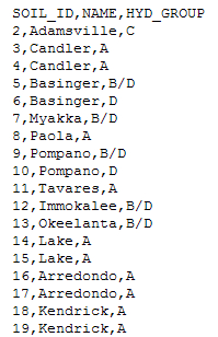
The first page of the Curve Number Calculator is used to assign hydrologic groups based on the soil GIS layer and optionally soil names (for reporting purposes).  If the hydrologic soil groups and/or soil names are contained within a GIS field, then the "Use Soils GIS Attribute" radio buttons should be selected.  However, if this information is not contained in the GIS file, then we must use the soil GIS layer in conjunction with a lookup table to assign soil names and hydrologic groupings.  The soil lookup table is a CSV file that will typically contain a soil ID number in the first column (this will need to match a corresponding Soil ID number in the GIS file), the soil name and the soil hydrologic group. An example of an extract from a soil lookup table is provided below.

 

 

Our soil GIS layer does not contain any hydrologic group or soil name information.  Therefore, we must use the soil GIS layer with a lookup table.

 

Ensure that both "Use Soil ID and Lookup Table" radio buttons are selected on the "Soils" page.  Select the soils GIS layer (i.e., "soilmu_a_fl017.shp") from the left and right "GIS File" drop down boxes and select the "MUSYM" field from the "Soil ID Field" drop down boxes.  This is the GIS field that contains the soil ID numbers.

 

Next we must open the lookup table that contains the soil ID, soil name and hydrologic groupings by clicking the "Open Lookup Table" buttons.  Separate lookup tables must be opened for both the Hydrologic Groups and Soil Names.  This enables you to have separate lookup tables for hydrologic groups and soil names if desired. However, for our tutorial all of this information is contained within the one file so we can just open the same lookup table ("Soils ID, Names & Hyd Group.csv") twice. Now select "SOIL_ID" from the 'Lookup ID Column' drop down boxes to identify which lookup table column contains the soil ID numbers. Select "HYD_GROUP" from the 'Lookup Hyd Column' drop down box and "NAME" from the 'Lookup Name Column' drop down box to identify which lookup table columns contain the hydrologic groups and soils names respectively.  The completed "Soils Page" should look similar to that shown below.

 

 

 

Once the "Soils" page is completed, click the "Land Use" tab. The "Land Use" page is used assign detailed land use descriptions to our land use GIS file, which is useful for reporting purposes. The "Land Use" page is also used to assign runoff curve numbers to each land use description for the four different hydrologic groups (ie., A, B, C and D).

 

First select the land use GIS file (Land_Use.shp) from the 'GIS File' drop down box. Then select "Layer" from the 'Land Use Attribute' drop down box. This is the GIS field that contains the basic land use descriptions.  You should notice that all of the available land use descriptions will appear in a new column in the centre of the "Land Use" page.  Now we must correlate these basic land use descriptions with more detailed land use descriptions and their associated curve numbers. This is achieved using a land use / curve number lookup table. The land use / curve number lookup table is typically extracted directly from publications such as TR-55 and comprises a CSV file that contains a detailed land use description in the first column and curve numbers for hydrologic soil groups A, B, C and D in the second, third, fourth and fifth columns. An extract from a land use / curve number lookup table is provided below.  

 

 

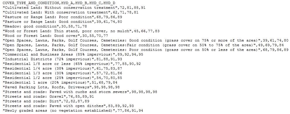
To open the land use / curve number lookup table, click the "Load Land Use / CN Table" button and locate the "FDOT Table T-7 - Selected Agricultural, Suburban, and Urban Land Use.csv" file and click "Open". Select "COVER_TYPE_AND_CONDITION" from the 'Land Use Column' drop down box.  This is the lookup table column that contains the detailed land use descriptions. Once you select this field, you should notice that a 'COVER_TYPE_AND_CONDITION' column has been added to the table in the centre of the "Land Use" page. If you click the table cell next to "COMMERCIAL" twice, a drop down box should appear as shown below.

 

 

All of the detailed land use descriptions from the lookup table will be available in this drop down box.  Scroll through the available detailed land use descriptions and select the one that most closely matches the "COMMERCIAL" land use description.  The "Commercial and Business Areas (85% impervious)" description should be appropriate.  Repeat this procedure for all of the land use descriptions until your "Land Use" page resembles that shown below:

 

 

If you would like to save the new lookup table that you have created in the centre of the page to use at a later date or for quality review purposes, you can click the "Save Lookup Table" button.

 

Once the "Land Use" page is completed, click the "Dual Hydrologic Groups" tab. The "Dual Hydrologic Groups" page is used to determine how an individual hydrologic group will be assigned for soils with dual hydrologic groupings (e.g., A/D, B/D and C/D). For soils with dual hydrologic groupings, the first letter applies where soils can be freely drained, while the second letter applies to undrained soils.

 

Four different options are available for calculating which hydrologic group letter to adopt:

 

1.Use First Group - This option will globally adopt the first hydrologic group letter. This may be suitable in a completely urban environment where drainage infrastructure would allow all soils to freely drain.

2.Use Second Group - This option will globally adopt the second hydrologic group letter (i.e., D). This may be suitable in a completely undeveloped environment where soils may not be able to freely drain.

3.Use First Group for the Following Land Uses - This option allows you to assign the first hydrologic group letter based on the overlaying land use by selecting a land use description from the drop down box (as defined on the "Land Uses" page) and clicking the "Add" button. Any land uses not added will be automatically assigned to the second hydrologic group letter.

4.Use Second Group for the Following Land Uses - This option allows you to assign the second hydrologic group letter based on the overlaying land use by selecting a land use description from the drop down box (as defined on the "Land Uses" page) and clicking the "Add" button. These will typically be undeveloped land uses (e.g., woods).  Any land uses not added will be automatically assigned to the first hydrologic group letter.

 

For this tutorial we will use option 4. Ensure that the "Use Second Group for the Following Land Uses" radio button is selected.  Select "Woods or Forest Land: Good Condition" from the drop down box and click the "Add" button. This will assign the hydrologic group 'D' to all soils with dual hydrologic groupings that underlie 'woods or forest land'.  All other soils with dual hydrologic groupings will be assigned the first hydrologic group.  The completed "Dual Hydrologic Groups" page should look like the following:

 

 

Once the "Dual Hydrologic Groups" page is completed, click the "Basin Select" tab. The "Basin Select" page allows you to specify if you would like to calculate runoff curve numbers for watershed boundaries that were derived in CatchmentSIM or whether you would like to import the watershed boundaries from an external GIS file. We will use the watershed boundaries that we have already developed in CatchmentSIM.  Ensure that the "Use basin boundaries in current CatchmentSIM Project" radio button is selected. Next click the "Run CN Calculator" button. CatchmentSIM will then create all of the necessary soil, land use and curve number raster files and add them to the CatchmentSIM project. This can be a time consuming process as the program needs to rasterise the existing soils and land use layers and create six new raster layers (e.g., basins, soil names, raw hydrologic groups, detailed land use, refined hydrologic groups and curve numbers).  

 

Before CatchmentSIM begins to rasterise the soil and land use GIS files, a Vector Data Set Operations form will appear.  This form allows you to specify which GIS entities in the soils and land use GIS files you would like to rasterize. We are interested in rasterizing all pixels that lie on a land use or soils polygon boundary as well as all pixels that are within a land use or soils polygon boundary. When the Vector Data Set Operations form appears, make sure the "Pixels on Polygon Boundary" and "Pixels within Polygon" check boxes are selected (as shown below) and click "OK".  

 

 

 

Once the raster calculations are complete, select the "Results" tab.  The results page allows you to review the curve number calculations for each watershed and export them to a CSV file.

 

On the "Results" page, we must first select which of the newly created raster layers we would like to select for reporting purposes. Select the raster layers as shown below:

 

 

Click "Select".  CatchmentSIM will intersect each of the selected layers and will list each unique land use and soil combination along with it's associated area and curve number in the main window as shown below.

 

 

At the moment, all watersheds are being displayed in the main table.  If you would like to review the curve number for a specific watershed, click on "All" in the 'Filter By' column next to Basin ID in the table located in the top right corner of the "Results" page.  This will open a drop down box listing all of the watersheds in the project.  Select a watershed (say 22) and click 'Refresh'.  The main table will be updated and will only show the curve number calculations for basin 22, as shown below.

 

 

The curve number calculations can be saved to a CSV file for reporting purposes. The curve number calculations can be grouped in a variety of ways.  However, the most common method is grouping by the watershed (or basin) ID.  Select "Basin ID" from the drop down box near the base of  the form and then click the "Save to CSV (group according to selected category)" button.  The resulting CSV file will look similar to the following when opened in Excel:

 

 

You will now notice that all of the newly created raster grids have been added to the list of available raster layers in the Layer Controller.  If you activate and move the "Curve Numbers" grid to the top of the raster layers list, make it 30% transparent and deselect the DEM layer, it should appear similar to the following.

 

 

This image shows how the curve numbers vary across the study area accordingly to the underlying soils types and land use categories. In this example, the lighter grey shades indicate lower curve number values (generally woods with soils belonging to the hydrologic group 'A') and the darker shades of grey indicate higher curve number values.

 

Any of the grid layers created as part of a CatchmentSIM project (e.g., DEM, curve numbers) can be exported from CatchmentSIM to an external GIS application (e.g., ArcGIS, MapWindow).  To export the curve number grid layer select Export >> Export Grid Data. Select the desired grid file format using the top drop down box and select "Curve_Numbers" from the bottom drop down box. Click "OK" to export the grid and then open the grid in your external GIS application. The following image was taken after loading the curve number grid layer into MapWindow.

 

 

 

conclusions

 

This tutorial has aimed to give you an introduction on applying CatchmentSIM to delineate a non-dendritic drainage system. Please feel free to experiment with the many other tools within the program and remember to check the website for software updates.

 

Feedback, ideas and questions are always appreciated and can be submitted via the website or user forums.