Download Tutorial 1 Data and Solution File
Tutorial 1 guides the user through developing a CatchmentSIM project for the Tweed River catchment, New South Wales, Australia. The tutorial will show you how to setup a CatchmentSIM project, sample DEM data from a web server, and utilising GIS input data to assist in the hydrologic modeling.
SETUP PROJECT
To begin any new project, the "Create new project" link can be selected from the opening startup screen, or if the startup screen is not displayed, by selecting the CatchmentSIM Drop Down >> New Project. This will display the new project dialogue, as shown below.
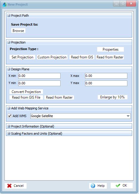
Enter any relevant information in the Project Information text fields (these can be left blank if you wish).
Click the 'Browse' button and enter the filename and save location of your project. This must be completed for all projects.
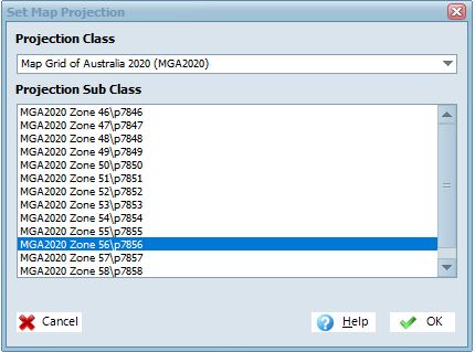
Now you must select an appropriate projection for the project by clicking the 'Set Projection' button. A projection is just a way to represent locations on the Earth's surface. In this tutorial, we will use "Map Grid of Australia 2000 (MGA2000)". To make this selection, choose Map Grid of Australia 2020 (MGA2020) from the top drop down menu. Now we must specify what MGA zone the catchment is located in. This particular catchment is located in Zone 56 so select "MGA2020 Zone 56\p7856" from the bottom drop down menu (as shown in image below).
 Additional Options for Defining Project Projection
The next step in setting up our project is to set the CatchmentSIM project extents. This is basically a large rectangle that fully encloses the proposed catchment extent. This step can be a challenge when the exact extent of the catchment is unknown. If you are uncertain it is best to overestimate the design plane extents.
The design plane extents can be specified manual by entering appropriate Xmin, Xmax, Ymin and Ymax values, or reading the extents from a raster or vector GIS layer. In the data folder for this tutorial, there is a KML file of Australian river basins and Google Earth Pro was used to manually save the Tweed River basin individually as a KML file.
Click Read from GIS File and select the Tweed River KML file. You will notice that the Xmin, Xmax, Ymin and Ymax values become populated, however, a keen GIS user will notice that these coordinates are in latitude/longitude. CatchmentSIM requires the design plane extent coordinates to be in the same projection as that which we specified when we click the "Set Projection" button. This is an issue as we have specified our project to be in MGA2020 Zone 56 projection. Therefore, a conversion from latitude/longitude needs to occur. CatchmentSIM is able to carry out this conversion by selecting the "Convert Projection" button. This will open a dialogue, firstly asking what the source projection is (this is the projection we are converting from), which is latitude/longitude (which on this occasion will be the default option) so we can simply click "OK". Another dialogue will appear asking what the destination projection we want to convert to will be. As we have previously selected MGA2020 Zone 56 as our project projection, CatchmentSIM will automatically select this projection and we can simply select 'OK' once again. You will now notice that the design extents are now in the correct coordinates.
To ensure our design plane completely covers the catchment extents, click the Enlarge 10% button and then click OK.
CREATE DEM
The next step in all projects is to setup a Digital Elevation Model (DEM) for our project. The DEM is a digital representation of the variation in terrain elevation across your study area. It is created by effectively dividing your study area into a grid of uniformly sized cell and assigning an elevation to each on these grid cells.
The creation of a suitable DEM requires some user discretion as to the appropriate grid size for the required application. For example, a large grid size could be used (e.g., >100metres) for a large, rural catchment where there are only very gradually variation in terrain elevation. However, for a small urbanised catchment with nuerous flow impediments (e.g., roadway embankment) may necessitate the use of a much small grid size (e.g., 2 metres).
For this project, we will utilise a 100m pixel size (100m x 100m grid cell size). To set this, select 'Create DEM >> Setup Blank DEM'.
The following dialogue will appear. We will leave the top radio button "1. DEM Extents" set on "Use Design Plane" as we are happy to use our project extents to also define our DEM extents. In the "DEM Cell Size" we will enter 100 in the input box. Click "OK".

ASSIGN DEM ELEVATIONS
In the previous step, we setup a DEM with a pixel size of 100m (i.e., a grid covering our entire project area with each cell measuring 100m x 100m in size). We now need to assign elevations to these pixels.
A variety of topographic data sources can be used to assign elevations to our "blank" DEM. This includes contours, raster DEMs, TINs as well as spot heights. Instructions on how to use contours is provided in Tutorial #2.
Where to find DEM information?
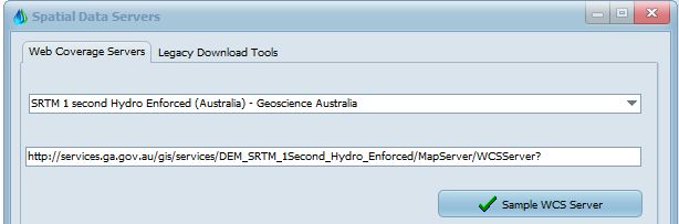
For this tutorial, we will utilise SRTM Raster DEM data from the web. To assign elevations from the SRTM data, navigate to Create DEM >> Download DEM Data. Select teh SRTM 1 second Hydro Enforced (Australia) option and Click "Sample WCS Server"
An inherit problem of raw DEMs is the fact that they are not instantly in a suitable condition to describe the flowpaths that exist across an area of interest. The major limitation that exists lies with "flat and pit" pixels. These pixels have an elevation the same as, or lower than, adjacent pixels, causing localised "sinks". This damages the flow connectivity and will ultimately result in unreliable flowpaths, stream and catchments. This is typically a result of "noise" in the input DEM information (e.g., vegetation).
CatchmentSIM includes a number of routines to remove the unwanted flat and pit pixels. The location and extent of these flat and pit pixels can be visualized by selecting the checkbox adjacent to the "Flat and Pits" in the left pane of CatchmentSIM. This left pane is the "view controller" and allows any CatchmentSIM layer to be turned on or off. The display order of layers can also be modified.
An image of the flat and pit pixels in our current project is shown below. Blue pixels indicate pits (pixels lower than adjacent pixels), and red indicates flat pixels (pixels with the same elevation as adjacent pixels). As can be seen, the majority of flats and pits are located along lower areas of the DEM (ie: where watercourses would lie), and the majority of flat pixels exist where the ocean/river would be expected.
IMPORT GIS FILES
Prior to carrying out any DEM "conditioning", we will add some GIS files to assist with the DEM conditioning process. For this tutorial, the GIS files include an ocean polygon and a coarse stream layer of the major watercourses in the area.
The ocean polygon can be added by selecting "GIS >> Ocean". Select the 'Aus_SWBD_Ocean.shp' file in the 'Data' folder and click "Open" and then "OK". A message box will appear stating that the *.shp file does not have any *.prj file and, therefore, a projection could not be determined. CatchmentSIM will convert input layers that are not in the same projection as our project to make sure the file is located in the correct position spatially. But it needs to know the projection of the input file before it can do this. Therefore, click "OK" and then select "Longitude/Latitude" from the top drop down box of the projection window (as we know the ocean layer is in latitude/longitude projection). Then click "OK". CatchmentSIM will perform all of the necessary coordinate conversion to ensure that ocean polygon layer overlays the project area correctly.
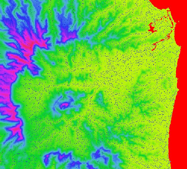
Now we will use the ocean polygon to lower the DEM cells below the ocean. This will help us condition the DEM by ensuring the ocean is the lowest point in our DEM. Select "DEM Conditioning >> Ocean >> Set Ocean Elevation". Enter a value of -10. The resulting DEM should look similar to that shown below.
Next, the watercourses layer can be added by selecting "GIS >> Streams". Navigate to the "Data/Streams" folder, select the "watercl.shp" file and click "Open". Click "OK" when the "Import Data" window appears. A message box will appear stating that the *.shp file does not have any *.prj file and, therefore, a projection could not be determined. Click "OK" and then select "Longitude/Latitude" from the top drop down box of the projection window. Then click "OK". The watercourses are now displayed in blue.
Any supported vector or raster layer can be added as a visual layer by selecting the green "+" button on the CatchmentSIM toolbar.

DEM MANIPULATION
It is important to note that there is no 'undo' function in CatchmentSIM, so any DEM manipulations made cannot be reversed. Hence, it is advisable to save your project prior to carrying out DEM manipulations to allow a 'fallback' project if you decide you are unhappy with the DEM modifications. Regular saving using the "CatchmentSIM Drop Down >> Save As" is recommended to allow you to revert to basically any stage of the CatchmentSIM project development process.
To allow effective catchment mapping and ensure flow can be routed from every pixel to the anticipated catchment outlet (in our case, the ocean), the DEM needs to be manipulated to allow continuous downstream flow path movement. The first DEM manipulation tool that can be used if you have watercourse data available is enforce streams. This can be complimented by Stream Burning, and finally, the Breaching Algorithm.
Firstly, we will "Enforce Streams" to help the condition the DEM. Enforcing streams ensures that all pixels underlying a stream/watercourse layer are always flowing "downhill". It will not alter pixel elevations where the downstream movement of water would naturally occur based on the DEM pixel elevations. However, if it encounters an adverse slope it will linearly lower the DEM elevation beneath the stream layer until it encounters another pixel with a lower elevation. To enforce streams, select "DEM Conditioning >> Enforce Streams". You should find that this will remove most of the flat and pit pixels underlying the watercourse layer. Note that this conditioning step is not essential, but is advisable if you have a reliable stream/watercourse layer.
Now we can apply the breaching algorithm to remove the remaining flat and pit pixels. This algorithm ensures flow from every pixel in the DEM can always move in a downstream direction to the lowest point in the DEM. In our project, we would expect that the ocean would provide the lowest point in our DEM (remember we previously set the ocean elevation to -10m to help ensure it was the lowest point in the DEM).
Select "DEM Conditioning >> Breaching Algorithm". Typically you can retain the default parameters. Click "Process Entire DEM". You will be asked if you wish to exclude oceans from the algorithm. Ensure that the oceans are excluded as this will decrease the processing time significantly (and we aren't really interested in mapping catchments across the ocean in any case).
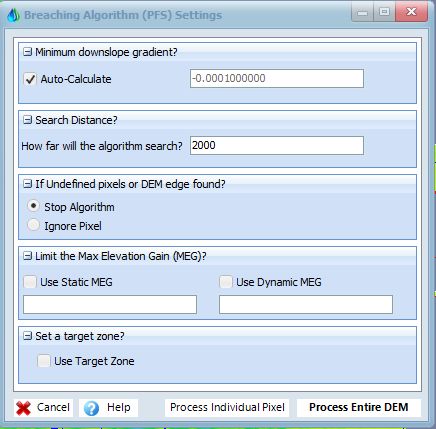
As the breaching algorithm processes, you can visually see the areas of the DEM's where the elevations have been modified to allow continuous flow paths, as indicated by the yellow lines that appear between flat and pit pixels. Further information on how the Breaching Algorithm finds the optimum downstream flow path can be found here. Once the algorithm has completed, you can remove temporary yellow "breach lines" by simply pressing 'F5', which is the refresh display hotkey.
We can now see if the DEM has been conditioned sufficiently by mapping a few flow paths from within out anticipated catchment and ensuring they are routed to our desired outlet location.
This can be completed using the "Draw Pixel Flow Path" feature available by "Flow Mapping >> Map Pixel Flow Path" (or F6 hotkey). Once you have selected this feature, left-click anywhere within the DEM and you should see a yellow flow path drawn indicating the flowpath that water will take from that particular pixel. If we click anywhere within the middle of our DEM (our area of interest), we should see that the flow paths all drain to the ocean.
Click to Enlarge Image
MAPPING CATCHMENT AND STREAMS
Now that we have an suitably conditioned DEM, we can map the catchment boundary and also create a detailed stream network.
In order to map a catchment, we need to first define a catchment outlet.
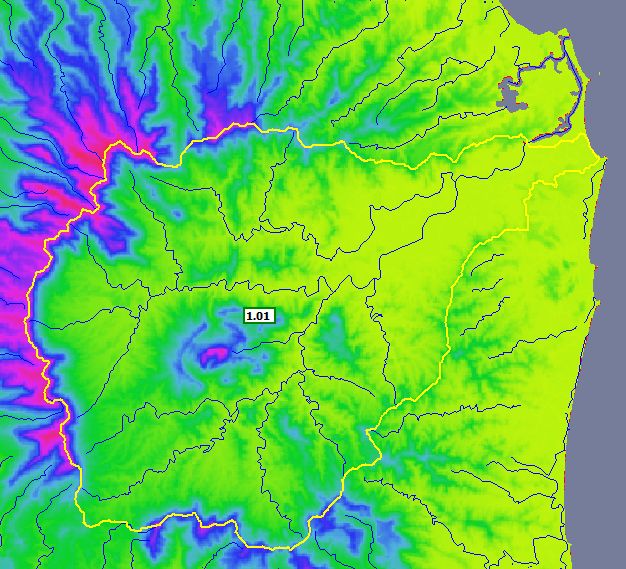
We can manually define a catchment outlet position by selecting "Subcatchments >> Draw Outlet". Draw a line at the location shown in the screenshot below (you may like to "zoom in" to this area using the zoom window or magnifying glass icons on the toolbar to make this a little easier). To do draw the outlet line, left click where you would like the outlet line to begin, left click again where you would like the outlet to end, and then right click to complete the outlet creation process. Make sure the line is orientated roughly perpendicular to the direction of flow and wide enough to 'catch' the flow that would pass by this position.
Alternative Outlet Definition Methods

Click to Enlarge Image

Click to Enlarge Image
Now we have defined an outlet for our catchment (the Tweed River). We will now get CatchmentSIM to map the catchment draining to this outlet by selecting "Subcatchments >> Map All". This is most time consuming algorithm as it needs to maps the path of flow from every pixel within the DEM to see which pixels ultimately drain through the outlet line that we have drawn.
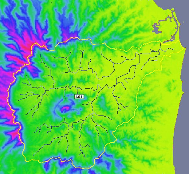
Once complete, the catchment should appear similar to that shown below.
Now we will map some streams. First, turn off the existing stream layer by unchecking the " " check box in the View Controller on the left side of the CatchmentSIM window. Now select "Flow Mapping >> Draw Streams". Check the "Restrict to Catchments" check box and enter a Stream Area Threshold (SAT) of "500 hectares". More about the SAT can be found here, but it is essentially the area must be draining to a particular point prior to a stream forming. The lower the SAT, the more detailed your stream network will be.

Alternative Stream Definition Methods
AUTOMATED CATCHMENT BREAKUP ROUTINE
Often catchments need to be broken down into smaller subcatchments. To assist in breaking up our catchment into subcatchments, CatchmentSIM has three different automated catchment breakup routines. These routines can be accessed via "Subcatchments >> Breakup Subcatchment".
Prior to describing the steps required to run the automated catchment breakup routine, it should be noted that additional outlets can be manually drawn utilising the same process as described above. The automated catchment breakup routine is aimed at breaking up large catchments where the manual specification of outlets would be time consuming.
We have multiple options for breaking up the catchment. Further information on the available breakup routines are available here.
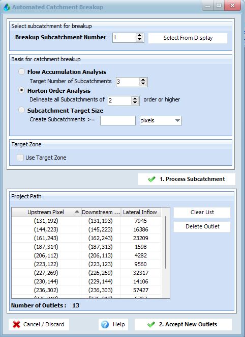
In this tutorial, we will use the Horton Order Analysis option to breakup the catchment. Do this by selecting the "Horton Order Analysis" radio button and entering a stream order or "2". Click the "Process Subcatchments" button followed by the "Accept New Outlets" button. Select "Yes" when prompted if you would like to refine the subcatchment. CatchmentSIM will analyse the input information and automatically place outlets at the junction of all stream with a Horton number of 2 or greater.
The resulting project should look similar to the following.

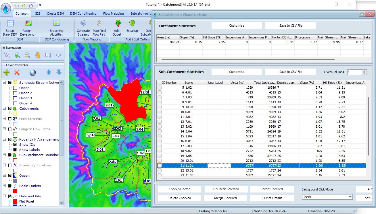
CatchmentSIM will automatically calculate a range of hydrologic properties for each subcatchment, including area, stream lengths, slopes. To view the subcatchment properties select "Subcatchments >> Subcatchment Manager". If you select a row in the subcatchment manager, the corresponding subcatchment will be highlighted in the main CatchmentSIM window.
EXPORTING SUBCATCHMENT BOUNDARIES, STREAM LAYER OR GRIDS TO OTHER SOFTWARE
CatchmentSIM allows you export all GIS and raster layers so they can be post-processed in other applications, or used in figure/report preparation. These export options is accessed through the "Export >> Export to GIS", or "Export >> Export Grid Data" respectively.
EXPORTING SUBCATCHMENT PARAMETERS TO HYDROLOGIC SOFTWARE
CatchmentSIM includes a Macro language package that will allow automated creation of input files for a range of Hydrologic software packages. For information on supported modelling packages, see the Macro Wizard dialogue and read the macro descriptions.
For this tutorial, we will run through the steps to output the required parameters for import into XP-RAFTS.
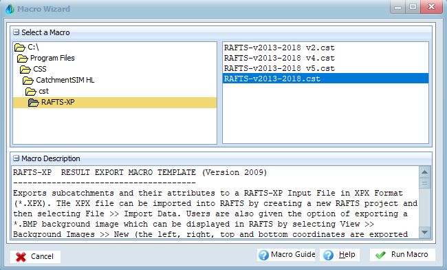
Go to "Export >> Macro Wizard". Here you will find "CatchmentSIM-Talk Macro Language" (CST) scripts for a range of different software as well as more generic reporting scripts (e.g., there is a script to automate GSDM Probable Maximum Precipitation calculations). Click the "RAFTS-XP" folder in the left pane. A list of RAFTS-XP CST script appears on the right hand pane and scripts are provided for various versions of RAFTS-XP. To export using a particular script, simply double click it and CatchmentSIM will prepare the output. You may be required to input/define some variables depending on the selected script and destination software package. A description of the macro is provided in the bottom pane to help you understand what the script does, help decide if the script is appropriate, and provide an explanation of what the export process is.
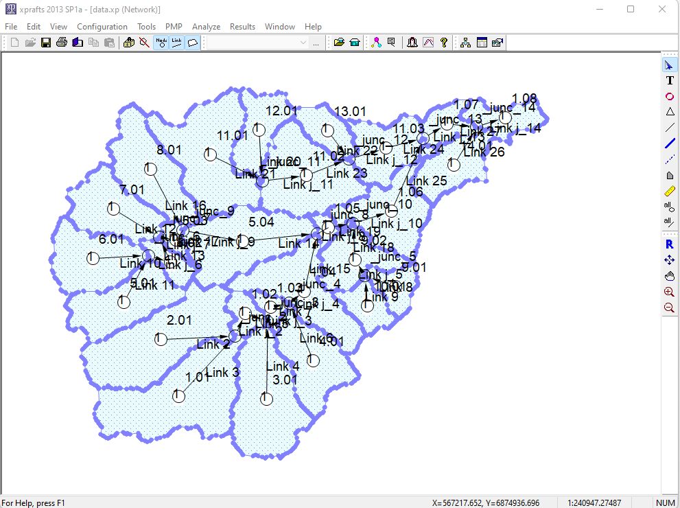
When running the script you will be asked a range of questions regarding how you would like the RAFTS model setup including junctions, routing and lag calculation options, default rainfall loss rates, roughness coefficient assumptions, subcatchment polygons and so on. Eventually, you will have an XPX file that can be imported into RAFTS. The process is simular for other models such as WBNM.
OPTIONAL EXERCISE
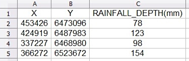
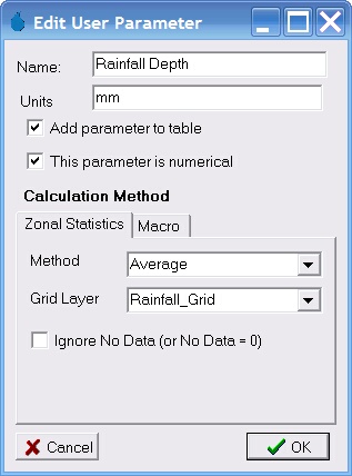
CREATE SPATIALLY VARYING RAINFALL GRID