Storm Injector Help

 

Summary

This exercise explores a theoretical catchment of 84 km2 with a flood detention basin at the outlet of subarea 3. It is based on one of the WBNM sample files (storage_partfull.wbn). The .wbn file preamble describes it as such:

An outlet structure (flood detention basin) is at the outlet of subarea 3. It is H_S type, ie you enter the culvert & weir dimensions and the discharge relation is automatically calculated. All culverts have inlet control. There are 3 outlets: 3 2400*1200 mm box culvert discharging to subarea 5; 2 1800 mm pipe culverts at elev 102.0 discharging to subarea 5; and a 12.0 m long weir at elev 105.0 discharging to OUTLET.

THE STORAGE IS INITIALLY FULL TO ELEVATION 102.0 M

The assumption around the initial storage elevation is a core part of this exercise. Firstly, we will create different versions of the wbn file with the storage starting full and empty and investigate if this assumption makes a difference to the design flow estimates when using the ensemble approach.

After this, we will do the same thing using Monte Carlo and see how the results compare.

Finally, we will use the Monte Carlo Variables to examine the results when using a stochastically generated number transformed through a distribution to cater for the uncertainty in the Initial Water Level (IWL). We will try both a Normal distribution of IWL as well as a Cumulative Density Function (CDF) approach.

The data for this exercise can be download from the links at Advanced Exercises.

 

Instructions

1.Import the project ex3_Storage_partfull.wbn. Click No since the project does not have real world coordinates.

2.This example is near Canberra so enter the coordinates of Latitude -35.3 and Longitude 149.13.

3.Click Yes to apply the NSW jurisdictional advice regarding continuing loss adjustment and the use of probability neutral initial losses.

4.For simplicity and due to a critical duration that may be less than 12 hours, we will use the Point Temporal Patterns. As such, click No when prompted to switch to Areal temporal patterns.

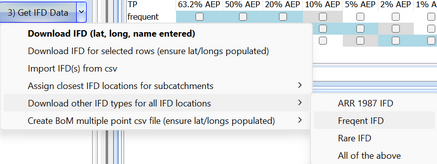
5.Click 3) Get IFD Data to get standard AEP rainfall data from the Bureau.

6.Click the button '3) Get IFD Data' drop arrow, then 'Download other IFD types for all IFD locations >> Frequent IFD' and then repeat for Rare IFD, in order to get all necessary rainfall data.
 

7.Let's do a critical duration analysis for the 1% AEP. Click the 1% AEP checkbox on the Point TP (ARR) tab and click 4) Create Storms.

8.Switch the model selector near Button 5 to 'WBNM (Internal)' and click 5) Prepare Model Runs, selecting the 'ex3_Storage_partfull.wbn' file.

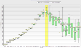
9.After running and processing these models (Buttons 6 and 7) on the Model Runs tab, you should see that the catchment has a critical duration of about 12 hours (Click Box Charts and click Chart in Compare Durations panel). Going forward, we will restrict our analysis to (6-18 hours). To do, this go to the Durations tab inside Selected Events panel on Storm Generator tab, right click and un-check all and then select only 6, 9, 12 and 18 hours.
 

   

10.Now, let's redo the analysis with the reduced number of durations for all standard AEPs. Switch to the Point TP (ARR) tab, right click and 'Select primary ensemble bins'. Click 4) Create Storms. Let's also do Rare events by clicking the Rare checkbox, select events 1 in 200 through to 1 in 2000 (no need to do 1 in 100 as we have the 1%). Importantly, click the drop arrow on '4) Create Storms' and select 'add to existing list of storms' (or it will overwrite the standard events).
 

 

11.Repeat buttons 5) Prepare Model Runs, 6) Run Models and 7) Process Results. You may get a Baseflow warning which you can ignore in this case. Once processed, you can click Box Charts and click Chart in Compare Events panel to view the range of results. You should see a full range of ensemble results with critical durations ranging from 6 - 12 hours.
 

 

12. Save this project as 'ex3-ensemble.esi'.

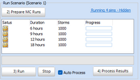
13.Next, let's  see if we can replicate these results with Monte Carlo. Switch to the Monte Carlo tab, click 1) Create MC Event, ensure the ARR Point TPs are selected in the Temporal Patterns tab (it may have defaulted to Areal TPs due to the catchment size), click 2) Prepare MC Runs and select the 'ex3_Storage_partfull.wbn' file. Click 3) Run.
 

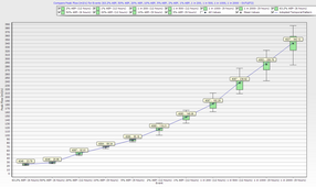
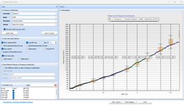
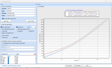
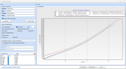
14.Note the speed of the MC approach since it is able to define all the AEP design flows in a single run. The tabular results can be seen in the results panel. The frequency curve can be seen using the Result Charts button. You can see the setting in the image below used to generate the plot. You should see a good match to the ensemble results until the very rare results such as 1 in 1000 where the MC distribution start to dip below the box and whisker plot quartiles.
 

 

 

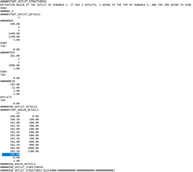
15.Next, we will generate different versions of the wbn text file with low (100m) and high (105m), IWLs to see if it makes a difference to the Monte Carlo design flow estimates. Open the 'ex3_Storage_partfull.wbn' file in a text editor and look at the Outlet Structures Block. The IWL is set near the end (Line 120) at 102.00. Change this to 100.00 and save the file as 'ex3_Storage_partfull_100.wbn' and then change to 105.00 and save the file 'ex3_Storage_partfull_105.wbn'. Now, you have two different models with low and high IWLs.
 

 

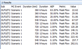
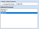
16.Create a new MC Scenario called 'Low IWL' and select the 'ex3_Storage_partfull_100.wbn' when clicking 2) Prepare MC Runs. Click 3) Run and wait for the results to process. Create another scenario called 'High IWL' and select the 'ex3_Storage_partfull_105.wbn' when clicking 2) Prepare MC Runs. Click 3) Run and wait for the results to process. You can compare the 1% Peak Flow results at the outlet as shown in the image below. It can be seen that the 1% AEP model peak outflow increases with a higher IWL assumption.
 

 

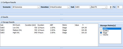
17.Scenario 1 is not the best name for our original scenario, you can rename it Medium IWL by right clicking on the scenario in the Selected Scenario panel and selecting 'Rename scenario' . You can also compare the stage results by configuring the results as shown in the image below. It can be seen that the 1% peak stage also increased based on the IWL assumption.
 

 

18.This trend can also be seen in the Results Charts by adding the results for Low, Medium and High IWL Scenarios one after another.
 

 

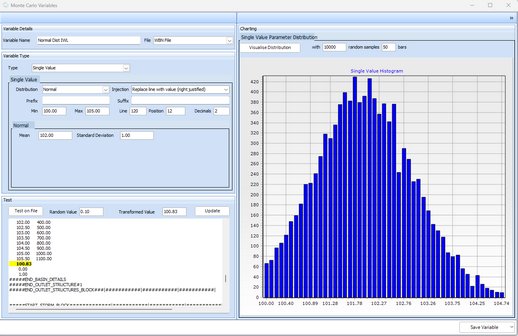
19.Now we know that the IWL in the flood detention basin does impact the design flow results. It is up to the practitioners judgment to adopt an IWL assumption. However, the Monte Carlo allows us to stochastically select this IWL from a distribution. Let's assume the IWL was a truncated Normal distribution with a mean of 102m and a standard deviation of 1m. Go to the Other Variables tab in the Parameter Setup panel and click Add New Variable. Configure it as shown below. Take note of the min, max, line no (as per text file), position (for insertion), decimals and injection type (replace line with value right justified). The distribution can be visualised with a stochastic sample using the Visualise Distribution button. The injection into the wbn model can be tested with the 'Test on File button' and selecting the wbn file. You should see that the value will be injected into line 120 to replace the existing value.
 

 

20.Click Save Variable. Then create a new scenario called 'Normal Dist IWL'. Check the option to include the 'Normal Dist IWL' variable. Then click 2) Prepare MC Runs and select the 'ex3_Storage_partfull.wbn' file (although any of the 3 versions should work since the IWL is being overwritten and this line is the only difference).
 

21. Click 3) Run and wait for the runs to complete.

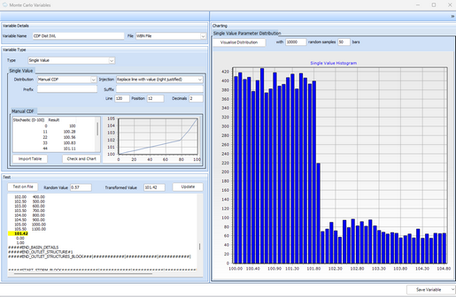
22.Alternatively, Let's assume we had good data on the IWL as defined by a Cumulative Density Function. Add a new variable and select the Manual CDF option in the Distribution combo box. Then click Import Table and select the 'CDF_Table.csv'. This csv is simply an excedance relationship for the basin. The other options should be set the same as for the previous normal distribution example.
 

23.Click Save Variable. Then create a new scenario called 'CDF Dist IWL'. Check the option to include the 'CDF Dist IWL' variable. Then click 2) Prepare MC Runs and select the 'ex3_Storage_partfull.wbn' file (although any of the 3 versions should work since the IWL is being overwritten and is the only difference).
 

 

24. Click 3) Run and wait for the runs to complete. When comparing the low, high and variable IWL (normal and CDF), you should see that the variable IWL values are between the Low and High IWL scenario options.
 

 

 

25.This exercise has aimed to demonstrate how Monte Carlo scenarios can be used to compare different model configurations and how Monte Carlo variables can be used to cater for uncertainty in IWL assumptions while maintaining AEP neutrality.

26.Save as 'ex3-complete.esi'