Storm Injector Help

 

Summary

This exercise focuses on applying the Monte Carlo approach to the projects created in Exercise 1 for the Coopers Creek catchment. Both standard and climate change scenarios will be created. The standard rare events and extreme rare event projects will both be examined to see how quickly and easily Monte Carlo can replicate these design flow estimates.

Representative events will be examined to see how Monte Carlo analysis could be used to input flows into a hydraulic model such as TUFLOW.

The data for this exercise can be download from the links at Advanced Exercises.

 

Instructions

This exercise builds on the same WBNM sample project 'CoopersCk.wbn', using the setup from Exercise 1. The goal is to generate Monte Carlo simulations up to the 1 in 2000 year AEP and compare it with FFA results.

1.Open the 'ex1-std-events.esi' project you create earlier, or the one provided in the course files.

2.Navigate to the Monte Carlo tab, enter the scenario name “std-no-cc” and click 1) Create MC Event
 

3.On the Rainfall tab, you should see the following settings: Rainfall Divisions: 50 divisions with 20 rainfall samples per division by default.
 

4.On the Losses tab, you should see the following settings.  Initial Losses is stochastically sampled where as Continuing Loss is not.
 

5.On Temporal Patterns Tab, select ARR Point TPs
 

6.The Other Variables tab should be left blank (we will discuss this in Exercise 3).

 

Settings tab: AEPs are generated from 1EY to 0.05%, covering up to the 1 in 2000 year event. This is based on the extents of the rainfall available in the selected IFD Locations in Storm Generator Tab.

 

7.Click 2) Prepare MC Runs. When prompted, select the file 'CoopersCk.wbn'

 

8.Click 3) Run. Wait for the simulation to finish. If results are not processed automatically, click 4) Process Results.

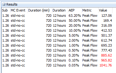
9.Now the results can be analysed. The Results table shows the peak flow estimates from the Line of Best Fit (LOBF). Red values suggest it is outside the accuracy limits of the method (refer to paper) and may require sampling of a larger rainfall domain (including rainfall rarer than the 1 in 2000 year AEP).
 

 
A chart such as the one below can be generated using the Results Chart button and configuring the options as per the options in the image. It shows that the MC LOBF fits within the ensemble box plot quartiles. The 12 hour event has again been identified as the critical duration.
 

10.Let's do another analysis for a climate change scenario. Create a new scenario called '2090-2.4-deg'. Then switch to the Storm Generator tab. Right click on the 2.4 degrees box (2090 / SSP2-4.5) and click 'Create Monte Carlo code'. You should then see climate change code added to the Custom Event Code in the Rainfall tab for the new Monte Carlo scenario.
 

   

 

11.Repeat buttons 2 - 4 and you should be able to review the revised results. You may notice that due to the Monte Carlo defining all AEPs in a single analysis, it is much quicker to undertake than using individual event custom event code as per Exercise 1.
 

 

 

12.The Coopers Creek catchment is reasonably well gauged with data from 1977-2025. A Bestfit analysis was done and can be imported for comparison. Right click on the FFA Data panel and click 'import >> BestFit RMC Series CSV', select the 'BestFit FFA.csv' file and then click Yes to import the Posterior Mode.
 

       

 

13.Update the chart by checking the 'Include FFA' checkbox, Clear Chart and then re-add the 'std-no-cc' scenario. It can be seen that the MC curve fits within the FFA confidence limits and quite closely follows the Posterior Mode results (yellow diamonds).
 

14.Close the Monte Carlo Chart form.

15.Representative Events are taken from the Monte Carlo sample where their value (such as peak flow) is close to the AEP of interest. For example, select only the 1.00% AEP and 'All Scenarios' in the Configure Results panel on the Monte Carlo tab. You should see 10 events populated in the Representative Events table. Currently, hydrographs have not been generated for these events so they will need to be re-run. Do this by clicking Run.
 

 
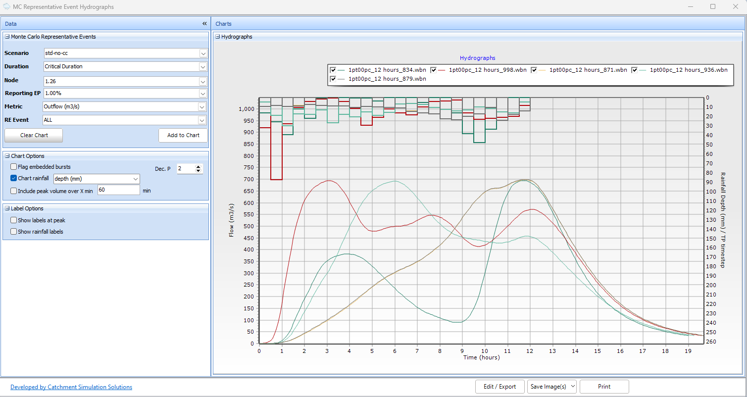
Once Run, we can Chart Hydrographs or export .ts1 files. Click Hydrograph Charts and then click Add to Chart. You should see that very different hydrographs have been presented but they all share a similar peak that closely matches the 1% AEP design flow estimate of ~ 700 for the standard non climate change scenario. These hydrographs could be used as an input to a hydraulic model.
 

16.Save the project as 'ex2-MC-std.esi'

17.Time permitting, you may like to undertake a similar comparison using the 'ex1-extreme-events.esi' project which will allow the Monte Carlo method to sample data all the way to the PMP estimate. You may get results like these.