CatchmentSIM Help

 

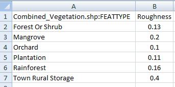
Now that our elevation grid, catchment boundary and stream network is defined, we must create an additional grid layer describing the variation in hydraulic roughness across our study area. The roughness coefficient is similar to a Manning's 'n' value adopted in hydraulic models. However, because the depths of flow across the majority of the catchment are generally quite shallow, the effective roughness of grass, shrubs etc is a lot more significant.  Therefore, the roughness coefficient values across the 2-dimensional domain in GSSHA are typically higher than a hydraulic model. The table below shows typical GSSHA roughness coefficient values for different land uses / vegetation types (Downer & Ogden, 2002).

 

The CatchmentSIM GSSHA interface provides a facility to incorporate a constant roughness coefficient value for all grid cells (useful for testing) or to define unique roughness coefficient values for each grid cell. For this example we will assign unique roughness values to each cell.

 

In order to define unique roughness value to each grid cell it is necessary to have a GIS or raster layer that describes the variation in land use / vegetation types across the catchment (or some other spatial dataset that can be used to describe the spatial variation in roughness values).  This may be a zoning map, a land use layer, a vegetation layer or a LiDAR intensity layer. Alternatively, land use/vegetation polygons can be defined by hand in a GIS or CatchmentSIM (GIS >> Draw Object >> Draw Impervious Area) based on aerial photography.

 

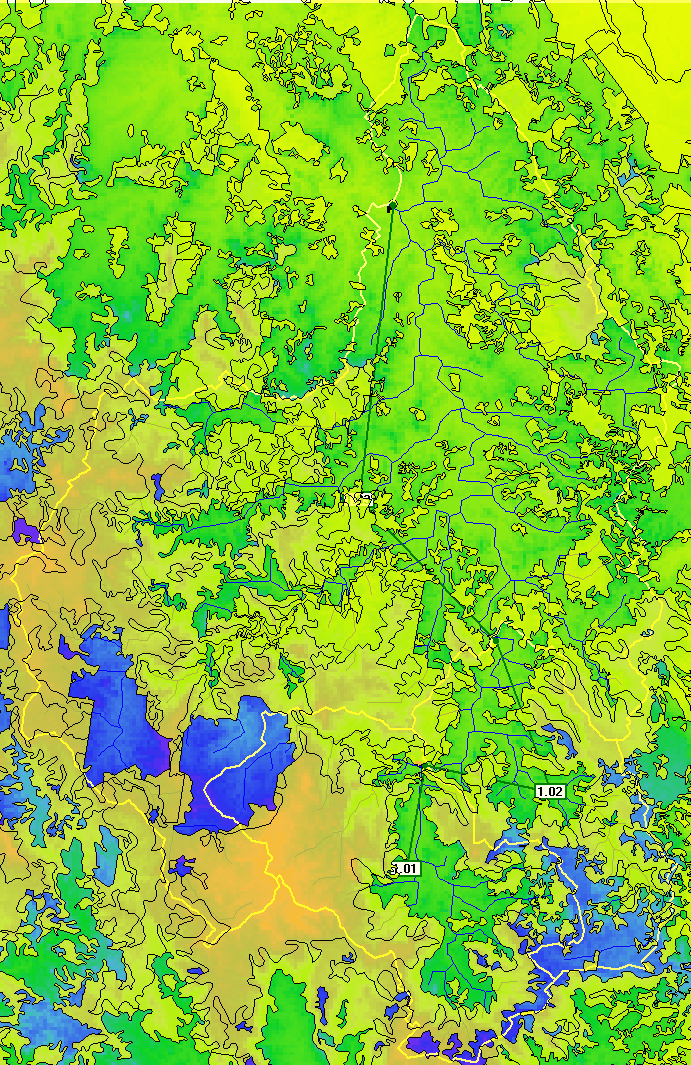
For this example, we will use 1:250,000 vegetation GIS layers to assign roughness values (the catchment is primarily undeveloped so a vegetation map will probably provide the best description of the variation in hydraulic resistance across the catchment). This information is available to download for free from Geoscience Australia's MapConnect page (http://www.ga.gov.au/mapconnect). Load the vegetation layer into CatchmentSIM by clicking the '' button on the toolbar, navigating to the 'Vegetation' directory and selecting the 'Combined_Vegetation.shp' file. The catchmentSIM project, should look similar to the following:

 

You will notice that there are significant areas where there are no vegetation polygons defined. If you look at these areas in Google Earth (GIS >> View in Google Earth), you can see that areas with no vegetation polygons define are typically cleared (i.e., areas that aren't cultivated or without native vegetation). The screenshots below show an area of the CatchmentSIM project and the image directly below is the same area in Google Earth. You can see that the polygons in the CatchmentSIM project typically coincide with forested areas, while areas outside polygons comprise pastures with minimal tree coverage.

 

 

Now we need to combine the vegetation types with a corresponding roughness values. This is achieved using CatchmentSIM's Raster Calculator with a lookup table. The Raster Calculator will effectively extract a vegetation type for each cell based on the vegetation layer that we have added. It will then search through the first column in the lookup table to identify that vegetation type and will then extract the corresponding roughness value from the second column of the lookup table. This roughness value will then be written to a new "Roughness" grid layer.

CatchmentSIM can assist with the development of the lookup table (Analysis >> Create Lookup Table), however, the lookup table for this example project has already been developed and is available in the 'VegetationCover' directory. This lookup table is also reproduced below:

 

Now open the Raster Calculator by selecting 'Analysis >> Raster Calculator'. If you are feeling confident, you can develop the necessary code to create the roughness grid. Alternatively you can just open the previously prepare 'Roughness.rcc' script by clicking the 'Load' button on Raster Calculator and navigating to the 'Script' directory. The Raster Calculator with the 'Roughness.rcc' script loaded is shown below:

 

Note that we have added an "if" statement in the raster calculator. This section of the script deals with the circumstance in which we have no vegetation polygons across certain areas (i.e., cleared areas). In such cases, it will assign a roughness value of '0.1', which corresponds to 'Grass and Pasture'. Also note that you will need to update the location of the lookup table ('S:\~Projects\GSSHA\CatchmentSIM\Tutorial #5-2\Script\VegetationLookup.csv' by default). This will need to be modified to reference the actual location of the 'VegetationLookup.csv' file on your computer.

 

Now to create the roughness grid click the 'RUN FUNCTION' button. When the Vector Data Set Operations dialog appears just press 'OK' (this handles the conversion of the vector vegetation GIS layer to a grid-based format).

 

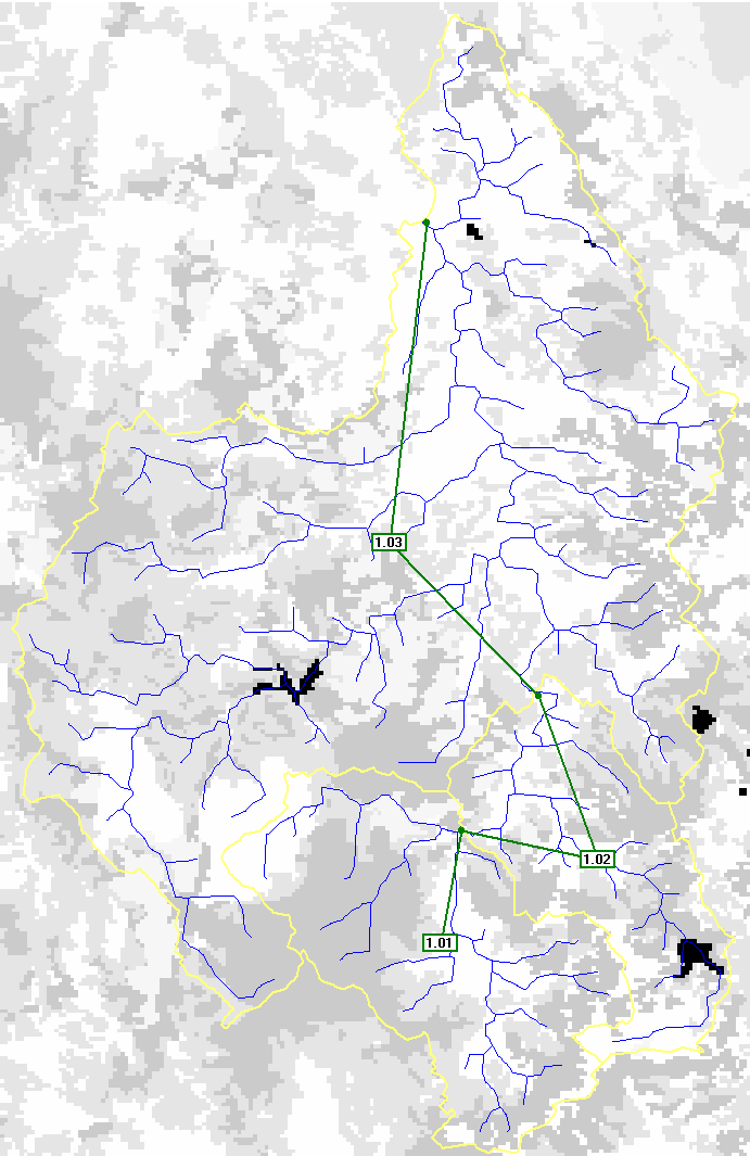
Once the script has completed running, you should find a new 'Roughness' grid layer in the View Controller on the left side of the CatchmentSIM window. Turn the layer on by checking the check bix. The layer should look similar to the following (note that the vegetation layers have been turned off in this image):

In the above image, areas with high roughness are assigned darker colours.

 

Note that for most projects, it will be necessary to refine the roughness values assigned based on the outcomes of model calibration. However, we have already calibrated these roughness values for you. So the roughness values should generate pretty reasonable results straight away. An easy way to complete model calibration is to apply a global multiplication factor to adjust roughness values up or down. Roughness values for individual vegetation types can then be adjusted individually to further improve the calibration.

 

We now have all the layers and information that we need to run a GSSHA simulation.