Storm Injector Help

 

The SorellCk_testDES.wbn file is distributed with WBNM 2020 and includes many storms to give an example of the range of ARR 2019 functionality within WBNM. The storm considered most relevant for verification was Storm 5 which was labelled:

 1% AEP  Dura and Pattern Spectrum  - Losses calc - ARF calc

That is, this storm was the 1% AEP event with automated calculation of ARF and initial losses.

 

Input Data

The wbn file references the following files

•SorellCk_CatchData2019.txt - An extract from the ARR Data Hub (ARR Data Hub Format)

•SorellCkBot.csv, SorellCkMid.csv, SorellCkTop.csv – IFD data for 3 gauges

•Southern_Slopes_Tasmania_Increments.csv – temporal patterns (ARR Data Hub Format)

 

Completing the Project in WBNM

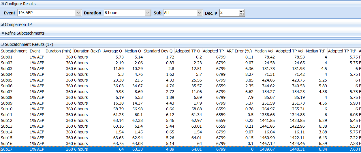
When running this file in WBNM 2020, the following results are generated:

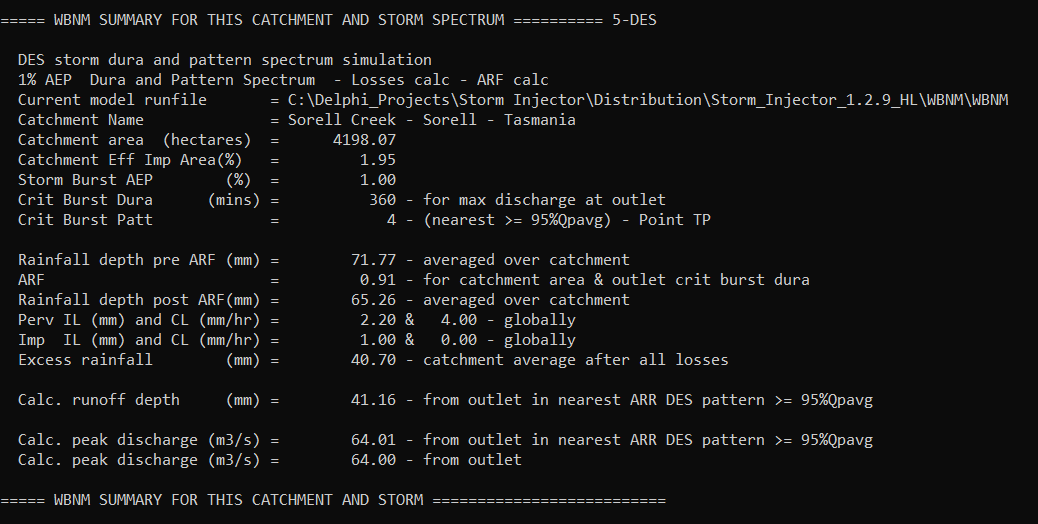
As shown above, the results are:

•360 min (6 hr) storm duration is deemed critical

•The ARF is 0.91

•The initial loss is 2.2mm

•The calculated peak discharge is 64.00 m3/s (average of all 6hr temporal patterns)

•The peak discharge of the adopted temporal pattern is 64.01 m3/s

 

The next section documents the steps to replicate these results using Storm Injector.

 

Completing the Project in Storm Injector

1.Import the .wbn file using the 1) Import Model button. Click Yes when prompted to convert the projection and select MGA Zone 55.

2.We wish to utilise the same data as WBNM wherever possible. As such, instead of downloading the ARR Data Hub information, click ‘2) Get Hub Data >> load text file’. Then select the ‘SorellCk_CatchData2019.txt’ file.

3.The ‘SorellCk_CatchData2019.txt’ file did not include the temporal patterns so these need to be manually imported. Right click on the grid in the Point TP Tab of the Temporal Patterns panel and select Import TPs and select the ‘Southern_Slopes_Tasmania_Increments.csv’ file.

4.Load the WBNM IFD data by clicking '3) Get IFD Data >> Import IFD(s) from CSV' and then select the 3 IFD files. When prompted to assign IFD locations to subareas based on X/Y coordinates, click Yes. However, ultimately, the weighting of the gauges will be overridden by the WBNM internal weighting.

5.To ensure consistency with WBNM, on the Settings tab ensure 1mm is set for the Impervious Initial Loss and 0mm for the Impervious Continuing loss. Also check the ‘Use WBNM Calc_RainGauge_Weights’ option in the WBNM Settings tab. This will allow WBNM to use its internal Thiessen Polygon rainfall weighting in preference to any IFD gauge assignments made in the Project Setup tab. Also ensure the 'Global Initial Loss minus Media pre-burst depth' option is selected in the Rainfall Losses panel.

6.Click the 1% AEP rare event in the Selected Events panel.

7.Click ‘4) Create Storms’.

8.You may need to set the Routing Increment in Max Inc (min) to 1 and click Recalculate. Higher routing increments will increase speed but can influence flows by a small amount.

9.Click ‘5) Prepare Model Runs’ and select the SorellCk_testDES.wbn file.

10.Ensure Auto-Process is selected and then Click ‘6) Run Models’.

 

In the model results, you can see that the 9 hour storm is found to be the critical duration for the catchment whereas WBNM 2020 found the 6 hour storm to be critical.

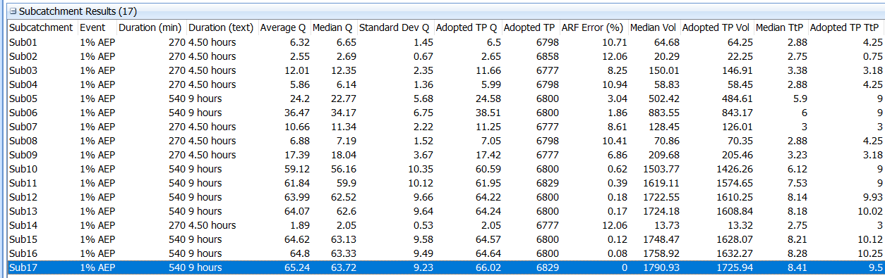
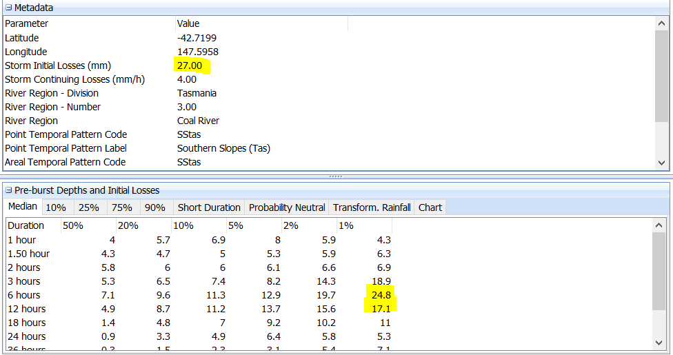
This difference is due to a different approach to the Median pre-burst between Storm Injector and WBNM 2020. Storm Injector interpolates the 9 hour pre-burst depth between the 6 and 12 hour depths (which determines an initial loss of 6.05mm) whereas WBNM 2020 adopts the 12 hour pre-burst depth  (which determines an initial loss 9.9 mm)

However, if you change the results to the 6 hour results, you should see that the average flow of 64.00 and Adopted TP flow of 64.01 is exactly matched.