Following the interpolation and hydrologic conditioning of the DEM, a flow mapping algorithm (Subcatchments >> Map All) can be applied to delineate subcatchment boundaries, determine the subcatchment network relationship and calculate geophysical subcatchment properties.
Theory
The flow mapping algorithm forms the basis of CatchmentSIM and is of vital importance to the quality of any GIS based hydrologic investigation. Most terrain analysis packages adopt the D8 method for flow mapping. However, CatchmentSIM utilises a modified version of Lea's (1992) method which has a number of advantages over the D8 method.
The modified version of Lea's (1992) algorithm calculates a downslope flow angle for each pixel that can be anywhere in the range of 0-360 degrees. The flow direction angle is determined as the resultant flow vector from the combination of the steepest non-diagonal pixel flow vector and the next steepest adjacent non-diagonal vector as outlined in Figure 17.
Figure 17 : Calculation of Flow Direction
Flow from each pixel is then mapped through all downslope pixels until a subcatchment outlet (or DEM boundary) is reached. The algorithm treats the flow path as a line and records the entry and exit points of the flow path through all pixels as a vector quantity such as illustrated in Figure 18.
Figure 18 : Vector Flow Path
As shown above, the described algorithm considers flow as a vector quantity flowing through a raster DEM. This technique has distinct advantages over more common approaches which consider flow as a raster quantity. In particular, it allows a greater representation of flow direction over hill-slopes and has greater sensitivity to flow divergence or convergence. For example, Figure 19 depicts parts of the CatchmentSIM flow paths mapped for 9 neighbouring pixels.
Figure 19 : Path Mapping Capabilities of CatchmentSIM
The distribution of flow paths can be seen in the lower right pixel in Figure 19 where flow paths from upstream pixels are distributed between both of this pixel's downslope pixels, based on where the flow paths entered the pixel. This cannot be accommodated in raster based flow mapping techniques and allows for a more reliable representation of flow distribution, and calculated drainage-path length / slope statistics. CatchmentSIM's flow mapping algorithm is analysed in more detail in the following section.
Comparison of Flow mapping Methods
Since the flow mapping algorithm is of vital importance to CatchmentSIM's algorithms it is worth comparing it to the commonly applied D8 method utilised by most other terrain analysis packages. The key disadvantage of the D8 method is it "snaps" flow to one of eight directions (whereas CatchmentSIM's flow algorithm can be any angle 0-360°). The approximation of drainage area to 22.5 degree increments might seem like a small loss in accuracy but this error can propagate over an area of consistent slope as demonstrated in Figure 20.
Figure 20 : Propagation of D8 Error Downslope
This type of error can also be observed in real catchments. For example, the flow paths generated by the D8 algorithm and the CatchmentSIM algorithm for 6 sample points in a catchment are compared in Figure 21, superimposed over the contours used to interpolate the DEM.
Figure 21 : D8 Flow Paths vs CatchmentSIM Algorithm
Figure 21 shows that significant deviations in the calculated flow paths exist for several of the sample points. The tendency of the D8 method to snap to cardinal or diagonal directions due to its limitation of eight potential directions can be clearly seen in the lower left sample points. In these cases the D8 flow paths are snapping to 45 degree lines since this is the closest approximation to local slope that the D8 algorithm can accommodate. The CatchmentSIM flow paths originating from these sample points flow more perpendicularly to the contours. Consequently, they are more hydrologically correct.
The effect of the errors associated with the D8 method can be seen to follow through into subcatchment delineation. The subcatchment boundary delineated from the same outlet point using the D8 and CatchmentSIM flow mapping algorithm is shown in Figure 22.
Figure 22 : Basin Delineation, D8 Method vs CatchmentSIM
The tendency of the D8 method to snap to diagonal and cardinal directions can again be seen in Figure 22, where the D8 generated boundary is biased towards the 45° angle and does not correctly identify the ridge line between the stream confluences. As shown in Figure 22, the two algorithms converge when they reach more defined ridge lines with stronger contour curvature. As such, the error introduced by the D8 method will be more pronounced in the outlet areas of subcatchments. The significant problem with quantifying this error is that it will be a function of the size of the subcatchment being delineated. This is because the length of the subcatchment boundary segment that does not follow major ridge lines will become a larger proportion of the total subcatchment boundary as subcatchment area decreases. As a result, the proportional error associated with the D8 method will become more pronounced the higher the discretisation of the catchment. This is an undesirable attribute of the method because higher catchment discretisation is usually undertaken to facilitate more accurate hydrologic modelling. Thus, if the D8 method is being applied then a user may inadvertently be introducing greater errors while attempting to gain greater accuracy.
Another shortcoming of the D8 method its underestimation of contributing areas in small subcatchments. An example of this is illustrated in Figure 23, which displays the D8 calculated upstream subcatchment for a single pixel. As shown, the combined area of the upstream pixels is only 50% of the real contributing area of the pixel (as indicated by the black border). This error varies from a factor of 0 (in cardinal directions) to 2 (in diagonal directions).
Figure 23 : D8 Contributing Area Calculation Error
The D8 method is not very successful at realistically representing flow convergence or divergence over hillslopes. This is due to the limited available flow directions available for each pixel. This causes the algorithm to effectively overlook or alternately, exaggerate subtle curvature of the DEM. For example, changes in flow direction that range between -22 to 22 degrees over a hillslope (a 44 degree range) that may be due to a small tributary will be ignored by the D8 method since all pixels will have their flow allocated to the immediately northward pixel. In contrast, minor (and possibly anomalous) changes in flow direction between 22 to 23 degrees will effect the D8 flow direction for the pixels, causing convergence when it is probably unnecessary. The effect of these problems is best shown in the stream networks that are generated used the D8 method, which is shown in Figure 24.
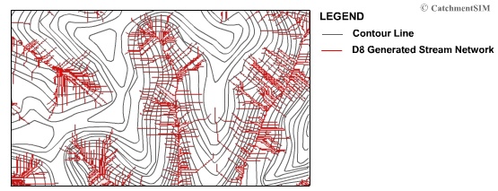
Figure 24 : D8 Parallel Streams
This figure shows the stream network generated using the D8 method on a sample DEM. Pixels are designated as streams when the number of upstream contributing pixels is greater than a specified value (Stream Area Threshold). The stream network relationship indicates many parallel streams in areas where contour curvature indicates flow convergence should exist. It can also be seen that the D8 method's failure to represent convergence has artificially raised the calculated drainage density in the region. These errors could seriously effect the calculation of geo-statistical quantities and subcatchment drainage path characteristics.