The DEM interpolation (Create DEM >> Interpolation Tools >> Interpolate Remaining Areas) phase refers to the calculation and assignment of elevations for all DEM pixels that remain unassigned following the source data rasterisation and watercourse interpolation phases.
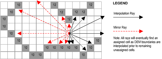
CatchmentSIM uses an interpolation algorithm based on a distance weighted average of a series of linear interpolations along a user-designated number of cross-sections taken through each pixel. For example, the interpolation regime shown in Figure 9 exhibits a 16 ray interpolation sequence. The 180 degree arc is divided into 8 increments and interpolation rays are initiated at the appropriate angles. All rays are paired with a mirror ray which travels in the opposite direction (ie., + 180 degrees).

\
Figure 9 : Interpolation of Digital Elevation Model
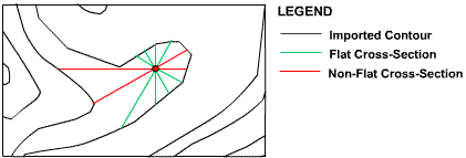
Once an interpolation ray and its corresponding mirror ray both intersect pixels with assigned elevations, linear interpolation is applied to determine the pixel elevation for that particular interpolation and mirror ray combination. The final value for the pixel is based on a weighted average of all the cross-section interpolations. The individual cross-section weights are based on the inverse of the distance between the located assigned pixels for the cross-section. During the algorithm development process it was found that flat cross-sections should be discounted (smaller weights) since they were over-flattening the topography in certain situations. An example of this can be seen in Figure 10.

Figure 10 : Flat Cross-Section Discounting Scenario
As illustrated in Figure 10, the non-flat cross-sections shown in red have the longest lengths and would consequently be given the smallest weights. However, due to the apparent ridge line evidenced by the contours, these cross-sections are more representative of the actual terrain and should be given more dominant weights than the surrounding flat cross-sections. These situations are accommodated by giving all flat cross-sections a discounting factor (FB) in their weight calculation as shown in Equation 1.
 (Equation 1)
In Equation 1, WN is individual cross-section weighting, DN is the distance between the assigned DEM pixels and FB is the flat cross-section discounting factor which is assigned the value of 1 except in the case of flat cross-sections where it is set at 10. This value was determined by empirical evaluation and visual analysis of the generated surface.
The final elevation of the pixel is calculated as shown in Equation 2 where WT is the sum of all individual weights and ZN is the linearly interpolated elevation for each individual cross-section
 (Equation 2)
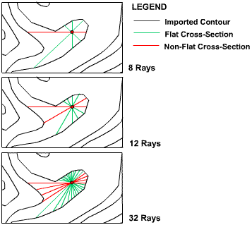
CatchmentSIM allows the user to designate the number of interpolation rays (and mirror rays) that are used to interpolate the pixel elevation. Increasing the number of rays will increase the accuracy of the interpolated surface as well as the computational demands of the algorithm. Figure 11 illustrates the advantages of increasing the resolution of the DEM interpolation algorithm.

Figure 11 : Increasing Resolution of DEM Interpolation
It can be seen in Figure 11 that the 32 ray interpolation algorithm has four non-flat cross-sections which will realistically represent the expected ridge line in the area. Ultimately, the best solution is reached when a cross-section alignment is found that is normal to the intersected contour lines, thus is approximately equal to local aspect. The 8 ray algorithm almost missed finding a non-flat cross-section, which would have resulted in a calculated elevation equal to the lower contour value. If there is no linear segment that can be found to construct a non-flat cross-section then an ITL can be used to correctly represent the ridge line. It is recommended that users adopt the maximum number of rays that their time requirements can accommodate. The relationship between number of rays and algorithm run time is directly linear (ie., twice as many rays will take twice as long). Algorithm run time will also increase with total grid pixels and sparsity of contour and watercourse data, since the search rays will need to travel further to find assigned pixels.